This repository is for SCOR Datathon held from November 2019 to February 2020 in Paris. SCOR is a tier 1 reinsurance company in the world. During this 4 months, we processed real open data, NHANES and NHCS, and built models to predict health risks of a person in U.S.
Our business problem identification
We have identified 2 biggest business problems for insurance and re-insurance companies; frauds and increase cost from chronic diseases.
With the growth of middle class and urbanisation, sedentary lifestyle is becoming more common across the world. This leads to an accerelation of costly chronic diseases.
Health care payers are seeking for solutions to decrease their premium cost not only by predicting one’s health risks to set correct premium, but also by improving one’s health; the longer the people without health problems, the cheaper the health cost that the payers pays.
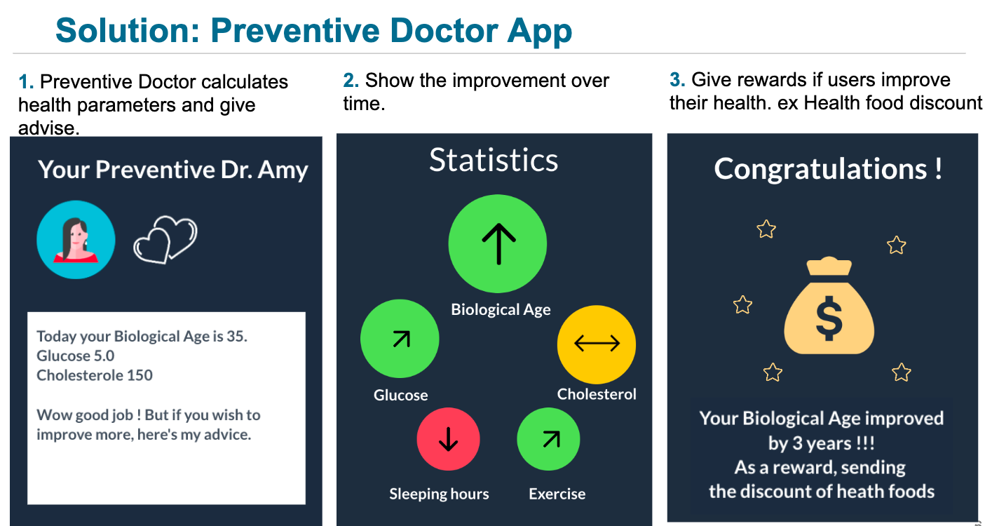
Our solutions
We have created a flask application to predict one’s diabetes risk, level of glycohemoglobin and cholesterol, and suggest how one can decrease the risk to specific level.
For example, we can say, to decrease the risk to 50% to 20% , we can suggest the person to walk 10 minutes more or sleep 1 hour longer per day.
Main Models for our application
Cox.PH to identify key features for health risks
Kaplan Meier to visualize survival curve for each indicators
Gradient Boost Regression to predict Glycohemoglobin and Cholesterol level of a person
Xgboost Classification to predict diabetes
SHAP value to calculate the marginal effect of certain variables to diabetes
Random Survival Forest to identify the probability change considering given age and other parameter change.
Configuration script
bash /home/pi/freezeralarm/configure.sh
Paste in Twilio and Adafruit credentials when prompted
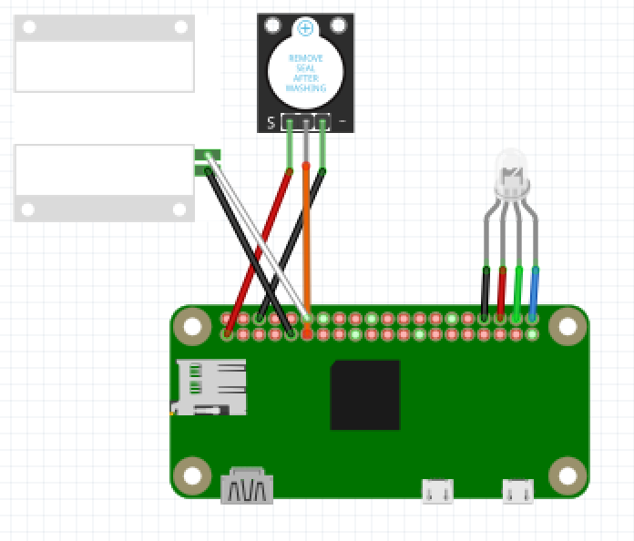
Single Door Alarm
Use singledooralarm.py
Connect the buzzer
Connect Pi 3.3V to Buzzer +
Connect Pi Pin 17 to Buzzer –
Connect Pi Ground to Buzzer N
Connect the door sensor, doesn’t matter which wire goes where
attach one wire to Pi Ground
attach the other wire to Pi Pin 18
Connect the LED
attach Pi Ground to black wire
attach Pi Pin 16 to the red wire
attach Pi Pin 20 to the green wire
attach Pi Pin 21 to the blue wire
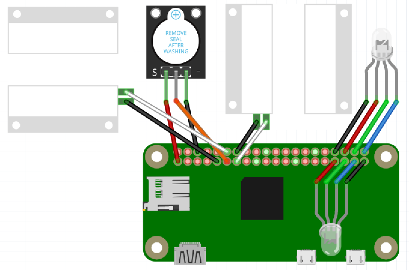
Double Door Alarm
Use doubledooralarm.py
Connect the buzzer
Connect Pi 3.3V to Buzzer +
Connect Pi Pin 17 to Buzzer –
Connect Pi Ground to Buzzer N
Connect the door sensors, doesn’t matter which wire goes where
Attach the first door sensor
attach one wire to Pi Ground
attach the other wire to Pi Pin 18
Attach the second door sensor
attach one wire to Pi Ground
attach the other wire to Pi Pin 27
Connect the LEDs
attach Pi Ground to black wire
attach Pi Pin 16 to the red wire
attach Pi Pin 20 to the green wire
attach Pi Pin 21 to the blue wire
attach Pi Ground to black wire
attach Pi Pin 13 to the red wire
attach Pi Pin 19 to the green wire
attach Pi Pin 26 to the blue wire
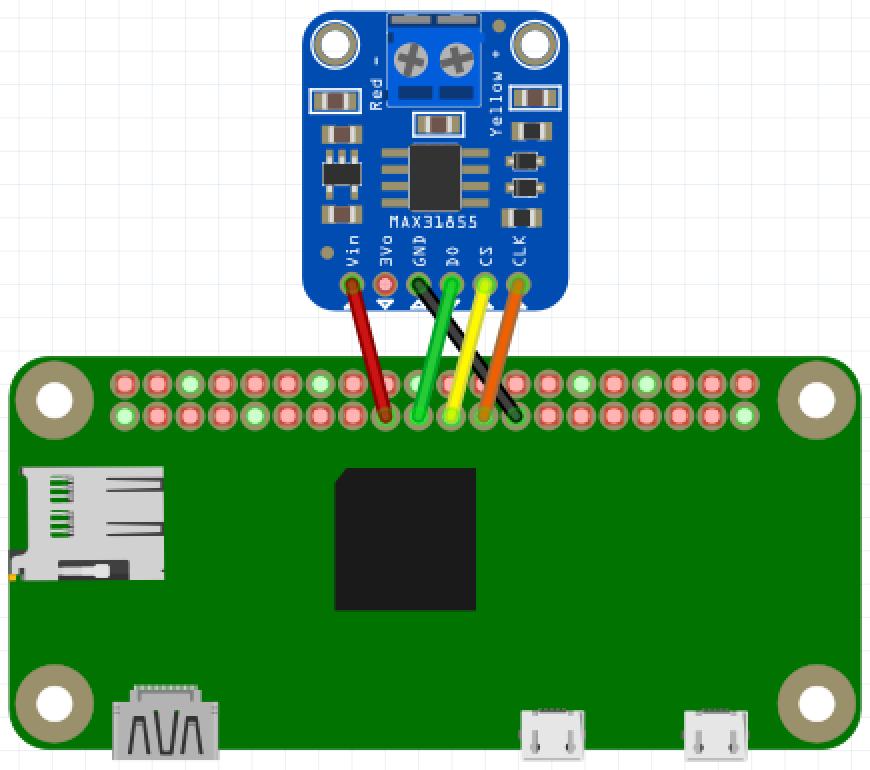
Temperature Monitoring
Use tempiodata.py
Connect the MAX31855
Connect Pi 3.3V to MAX31855 Vin
Connect Pi GND to MAX31855 GND
Connect Pi GPIO 10 to MAX31855 DO.
Connect Pi GPIO 9 to MAX31855 CS.
Connect Pi GPIO 11 to MAX31855 CLK.
An efficient array storage engine for managing multi-dimensional arrays.
The MSDB software provides various compression options to make the array compact, and it also can fastly perform queries on them.
This library can be embedded any C++ projects.
It adapts Array Functional Language (AFL), which is widely used in many array databases, instead of SQL.
This is a simple package to compute different metrics for Medical image segmentation(images with suffix .mhd, .mha, .nii, .nii.gz or .nrrd ), and write them to csv file.
BTW, if you need the support for more suffix, just let me know by creating new issues
Summary
To assess the segmentation performance, there are several different methods. Two main methods are volume-based metrics and distance-based metrics.
Metrics included
This library computes the following performance metrics for segmentation:
Note: These metrics are symmetric, which means the distance from A to B is the same as the distance from B to A. More detailed explanication of these surface distance based metrics could be found here.
Evaluate two batches of images with same filenames from two different folders
labels= [0, 4, 5 ,6 ,7 , 8]
gdth_path='data/gdth'# this folder saves a batch of ground truth imagespred_path='data/pred'# this folder saves the same number of prediction imagescsv_file='metrics.csv'# results will be saved to this file and prented on terminal as well. If not set, results # will only be shown on terminal.metrics=sg.write_metrics(labels=labels[1:], # exclude backgroundgdth_path=gdth_path,
pred_path=pred_path,
csv_file=csv_file)
print(metrics) # a list of dictionaries which includes the metrics for each pair of image.
After runing the above codes, you can get a list of dictionariesmetrics which contains all the metrics. Also you can find a .csv file containing all metrics in the same directory. If the csv_file is not given, the metrics results will not be saved to disk.
Evaluate two images
labels= [0, 4, 5 ,6 ,7 , 8]
gdth_file='data/gdth.mhd'# ground truth image full pathpred_file='data/pred.mhd'# prediction image full pathcsv_file='metrics.csv'metrics=sg.write_metrics(labels=labels[1:], # exclude backgroundgdth_path=gdth_file,
pred_path=pred_file,
csv_file=csv_file)
After runing the above codes, you can get a dictionarymetrics which contains all the metrics. Also you can find a .csv file containing all metrics in the same directory.
Note:
When evaluating one image, the returned metrics is a dictionary.
When evaluating a batch of images, the returned metrics is a list of dictionaries.
Evaluate two images with specific metrics
labels= [0, 4, 5 ,6 ,7 , 8]
gdth_file='data/gdth.mhd'pred_file='data/pred.mhd'csv_file='metrics.csv'metrics=sg.write_metrics(labels=labels[1:], # exclude background if neededgdth_path=gdth_file,
pred_path=pred_file,
csv_file=csv_file,
metrics=['dice', 'hd'])
# for only one metricmetrics=sg.write_metrics(labels=labels[1:], # exclude background if neededgdth_path=gdth_file,
pred_path=pred_file,
csv_file=csv_file,
metrics='msd')
By passing the following parameters to select specific metrics.
The two images must be both numpy.ndarray or SimpleITK.Image.
Input arguments are different. Please use gdth_img and pred_img instead of gdth_path and pred_path.
If evaluating numpy.ndarray, the default spacing for all dimensions would be 1.0 for distance based metrics.
If you want to evaluate numpy.ndarray with specific spacing, pass a sequence with the length of image dimension as spacing.
labels= [0, 1, 2]
gdth_img=np.array([[0,0,1],
[0,1,2]])
pred_img=np.array([[0,0,1],
[0,2,2]])
csv_file='metrics.csv'spacing= [1, 2]
metrics=sg.write_metrics(labels=labels[1:], # exclude background if neededgdth_img=gdth_img,
pred_img=pred_img,
csv_file=csv_file,
spacing=spacing,
metrics=['dice', 'hd'])
# for only one metricsmetrics=sg.write_metrics(labels=labels[1:], # exclude background if neededgdth_img=gdth_img,
pred_img=pred_img,
csv_file=csv_file,
spacing=spacing,
metrics='msd')
About the calculation of surface distance
The default surface distance is calculated based on fullyConnected border. To change the default connected type,
you can set argument fullyConnected as False as follows.
In 2D image, fullyconnected means 8 neighbor points, while faceconnected means 4 neighbor points.
In 3D image, fullyconnected means 26 neighbor points, while faceconnected means 6 neighbor points.
How to obtain more metrics? like “False omission rate” or “Accuracy”?
A great number of different metrics, like “False omission rate” or “Accuracy”, could be derived from some the confusion matrics. To calculate more metrics or design custom metrics, use TPTNFPFN=True to return the number of voxels/pixels of true positive (TP), true negative (TN), false positive (FP), false negative (FN) predictions. For example,
medpy also provide functions to calculate metrics for medical images. But seg-metrics
has several advantages.
Faster. seg-metrics is 10 times faster calculating distance based metrics. This jupyter
notebook could reproduce the results.
More convenient. seg-metrics can calculate all different metrics in once in one function while
medpy needs to call different functions multiple times which cost more time and code.
More Powerful. seg-metrics can calculate multi-label segmentation metrics and save results to
.csv file in good manner, but medpy only provides binary segmentation metrics. Comparision can be found in this jupyter
notebook.
If this repository helps you in anyway, show your love ❤️ by putting a ⭐ on this project.
I would also appreciate it if you cite the package in your publication. (Note: This package is NOT approved for clinical use and is intended for research use only. )
Citation
If you use this software anywhere we would appreciate if you cite the following articles:
Jia, Jingnan, Marius Staring, and Berend C. Stoel. “seg-metrics: a Python package to compute segmentation metrics.” medRxiv (2024): 2024-02.
@article{jia2024seg,
  title={seg-metrics: a Python package to compute segmentation metrics},
  author={Jia, Jingnan and Staring, Marius and Stoel, Berend C},
  journal={medRxiv},
  pages={2024--02},
  year={2024},
  publisher={Cold Spring Harbor Laboratory Press}
}
This repository will contain three different types of data structures:
Sentinel-based data structure
Dynamic data structure using malloc for memory allocation
Linked data structure using pointers to point to the next element in the structure
Sentinel-based Data Structure
The sentinel-based data structure is a type of data structure that uses a sentinel node to mark the beginning and end of the structure. The sentinel node is a special node that does not contain any actual data but is used as a marker to indicate the beginning or end of the structure. This type of data structure is often used in algorithms that need to search through a data structure, such as sorting algorithms or binary search.
Dynamic Data Structure using malloc
The dynamic data structure is a type of data structure that uses malloc to allocate memory dynamically. This means that the size of the data structure can be determined at run-time rather than at compile-time. This type of data structure is often used in situations where the size of the data to be stored is not known in advance.
Linked Data Structure using Pointers
The linked data structure is a type of data structure that uses pointers to link each element to the next element in the structure. Each element contains a data field and a pointer field that points to the next element in the structure. This type of data structure is often used in situations where the data needs to be accessed sequentially, such as in a queue or a linked list.
When the connect-mesh gateway is powered on and connected to the internet, it will show in the discovery list. Add the device.
Note: If the last step doesn’t work, the device may still be connected to your phone. Switch back to ‘Control mode’ on the dashboard, and a blue popup should appear allowing you to connect to the ‘cloud’.
Ensure Other Devices Are Connected:
Make sure you have other devices connected that you will need to control through Home Assistant.
Upload App Configuration to Cloud:
After making any changes in the app or completing the first setup:
Change to ‘Control mode’ in the app.
Navigate to Gateway > Cloud settings > Synced networks.
Click on the network upload button to sync your configuration with the cloud.
Troubleshooting
Lights on the Gateway:
BLE flickering: Not connected to the Connect Mesh app
Reset the gateway device with the physical button and try again.
Internet flickering: Not connected to the internet.
Check if the cable works and you are signed into an account on the app.
Step 2: Create an API Token
Make sure you signed into your Connect Cloud Account and ensure all gateway lights are on.
Go to Connect Mesh Cloud and sign in with the account you created in Step 1.
Navigate to the Developer Page (use this link as there’s no button).
Create a new API token:
Use the offset to change the expiration date (unit: MONTH, offset: 36, for 3 years).
Click on SET before creating the token.
Example token: CMC_ab12cd34_ef56gh78ij90kl12mn34op56qr78st90uv12wx34yz56ab78cd90ef12.
Step 3: Add Custom Repository in HACS
In Home Assistant Community Store (HACS), add this custom repository.
Install Häfele Connect Mesh.
Step 4: Add the Integration
Add the Häfele Connect Mesh integration.
Fill in the API token.
Select the network you want to add and submit.
You are all set!
To Do List
Add a way to change RGB color when API supports this functionality.
Resolve the issue where name changes through the app don’t appear in Home Assistant.
Investigate the possibility to see states when using a physical button.
Feel free to customize it further as per your needs.
This, of course, is not a “quick sort” because the original one is an “in place” algorithm that doesn’t require additional memory space allocation. This is a functional oriented expression that exemplarizes how expressive a “functional” orientation can be (You “express” that the sorted version of an array is, given one of it’s elements, the sorted version of the smaller ones, plus the item, plus the sorted version of the bigger ones).
As an enthusiastic newbie to the “D” programming language, I thought that D could affort this expressiveness too…
D has no support for destructuring as javascript has (remember de sorted([pivot, ...others])), but it has lambdas, map/filter/reduce support, array slices and array concatenation that allows you to write easily a similar expression:
note: D notation allows to write foo(a) as a.foo() or a.foo, this is the reason we can write sorted( array( something ) ) as something.array.sorted
note: sorted is a templated method (T is the type of the elements of the array): “under the scenes”, D compiler detects if the final used type is comparable (i.e.: it is a class with a opCmp method, or it is a numerical type, or …): yo don’t need to tell that T extends something like “IComparable” because D libraries are not “interface” based: D prefers to use “conventions” and check them using instrospection at compile time (D developers write compile-time code and run-time code at the same time: D allows you to mix them naturally).
Seeing the similarities, I assume (I really don’t know) that javascript and D versions are doing the same “under the scenes”:
The [...array1, ...array2, ...array3] javascript is equivalent to the array1 ~ array2 ~ array3 D code. That is, a new array is being generated as a result of copying the elements of the original 3.
The .filter!(...).array D code is using a “Range” to filter the elements and the “.array()” method to materialize the selected elements as an array. Internally, it is similar to the javascript code where .filter(...) iterates and selects the resulting elements and finally materializes the array
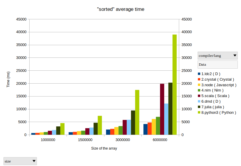
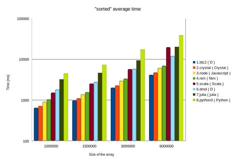
Wich one will perform better?
First surprise was Javascript (nodejs) version performs better than D (about 20% faster for 1_000_000 random Float64 numbers).
Javascript (node): 1610 ms
D (DMD compiler): 2017 ms
Fortunately, D has 3 compilers: DMD (official reference compiler), GDC (GCC based compiler) and LDC (LLVM based compiler).
D (LDC compiler): 693 ms !!!
That’s speed 🙂
After some tests, I realized javascript destructuring [pivot,…others] caused a performance penalty and I rewrote to a more efficient version (very similar to D syntax)
functionsorted(xs::Array{Float64, 1})::Array{Float64, 1}returnlength(xs) ==0?Array{Float64, 1}() :vcat(
sorted([x for x in xs[2:end] if x < xs[1]]),
xs[1],
sorted([x for x in xs[2:end] if x >= xs[1]])
)
end
This repository serves as a documentation of my journey through UB’s Information Technology program. It’s a practical, hands-on account of my experiences in coding and IT projects. From tackling coding challenges to exploring various programming languages, it’s a raw and unfiltered view of my growth as a programmer. No frills, just real progress.
This repository serves to chronicle my experiences and projects during my time in UB’s Information Technology program. It showcases my progress as a programmer, from coding challenges to complex IT projects.
File Structure
Folders are divided by semester, course, and assessment type.
2023-1 Fall Semester (August 2023 to December 2023)
[cmps1131] Principles of Programming 1
[cmps1134] Fundamentals of Computing
2023-2 Spring Semester (January 2024 to May 2024)
[cmps1232] Principles of Programming 2
2024-1 Fall Semester (August 2024 to December 2024)
2024-2 Spring Semester (January 2025 to May 2025)
2025-1 Fall Semester (August 2025 to December 2025)
2025-2 Spring Semester (January 2026 to May 2026)
2026-1 Fall Semester (August 2026 to December 2026)
2026-2 Spring Semester (January 2027 to May 2027)
Navigating Semesters, Courses, and Assessments
This repository is organized by semesters, courses, and assessment type. Here’s how you can navigate through the structure:
20XX-X: Click on the respective semester folder to explore the courses undertaken during that semester.
Course Name: Inside each semester folder, find individual course folders. Each course folder contains assignments and assessments.
Assessment Type: Inside each course folder, explore different types of assessment folders. These folders contain project files, assignments, and other materials related to the coursework.
License
This project is licensed under the MIT License – see the LICENSE file for details.
In this project, first a code for an image classifier is built with TensorFlow and a Keras model is generated, then it will be converted it into a command line application. the command line application takes an image and the trained Keras model, and then returns the top K most likely class labels along with the probabilities.
Goal
Classify images of flowers to 102 diffrent categories.
Data
A dataset from Oxford of 102 flower categories is used. This dataset has 1,020 images in the training and avaluation set, and 6,149 images in the test set.
Model
A MobileNet pre-trained network from TensorFlow Hub is used.
The model is used without its last layer, and some fully connected layers with dropout is added sequentially to be trained on the data.
A model using Conv2D and some fully connected layers with dropout is added sequentially to be trained on the data.
Code
The code is provided in the finding_donors.ipynb notebook file. the visuals.py Python file and the census.csv dataset file is used.
Run
In a terminal or command window, navigate to the top-level project directory finding_donors/ (that contains this README) and run one of the following commands:
It will print the top_k or 3 most probable predicted classes for the image. If the label_map.json is also given, the the name of each flower representing each class will be shown.


 https://github.com/cnai-ds/Datathon-Health-Risk-Prediction